3. Estimating Residues

After modal frequencies & damping have been estimated, modal residues (mode shape components) are estimated during a second curve fitting step.

• Execute Display | mooZ mooZ is the reverse of a Zoom operation in a Structure, Data Block, or Acquisition window. It restores the full display of the structure model in a Structure window, or the display of all of the M# data in a Data Block or Acquisition window. to restore the full graphics display.

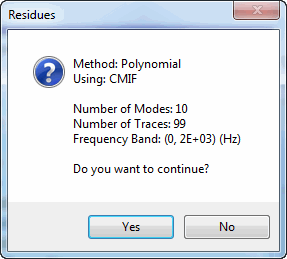
• Press the Residues button on the Residues, Save Shapes tab.

• Click on Yes in the dialog box that opens.

Residues Dialog Box.

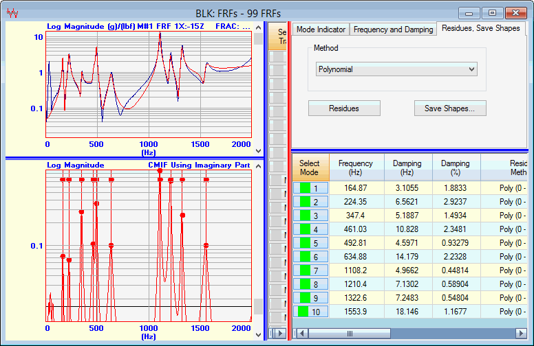
Estimates of residue magnitude & phase for all 10 modes and each FRF An FRF (Frequency Response Function) is a cross-channel frequency domain function that defines the dynamic properties of a structure between an excitation Force and the Response caused by that force. An FRF is defined as the ratio (Response DFT / Force DFT). The FRF is a special case of a Transfer Function, where the response is the numerator (Output) and the force is the denominator (Input). Trace are added to the Modal Parameters spreadsheet.

• Scroll through the M#s and release the mouse button to list the residues for the M# being displayed.

Residue Curve Fit of 10 Modes and 99 FRFs.

Fit Function

After the modal frequency, damping, & residue have been estimated, a red Fit Function is also overlaid on each Trace, as shown above.

• The Fit Function is calculated using the modal parameter estimates.

• If the modal parameters are accurate, then the Fit Function will lie on top of the FRF data.

Using the Band Cursor

If the Band Cursor One of the three types of cursors in a Data Block or Acquisition window. It is displayed as two vertical lines on each M#. Click & drag inside the band to move the Band cursor. Click & drag outside the band to move the nearest edge of the Band cursor. is displayed, curve fitting is done using data from within the cursor band  It is often more convenient to curve fit using several cursor bands to avoid noise or non-resonance peaks in the FRFs.

• Execute Curve Fit | Clear Fit Function, and click on Yes in the dialog box.

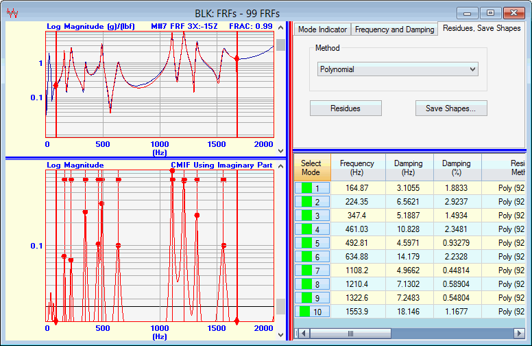
• Execute Display | Cursors | Band Cursor and drag the edges of the band to enclose the 10 resonance peaks, as shown below.

• Press the Residues button again, and click on Yes in the dialog box.

Notice that the red Fit Function is only displayed over the cursor band because only that data was used for curve fitting.  The residue estimates will also be slightly different when residue curve fitting is done in cursor bands instead of using all of the FRF data.

Residue Curve Fitting in a Cursor Band.